Data Locality and GPU Utilization in Multi-Node Training

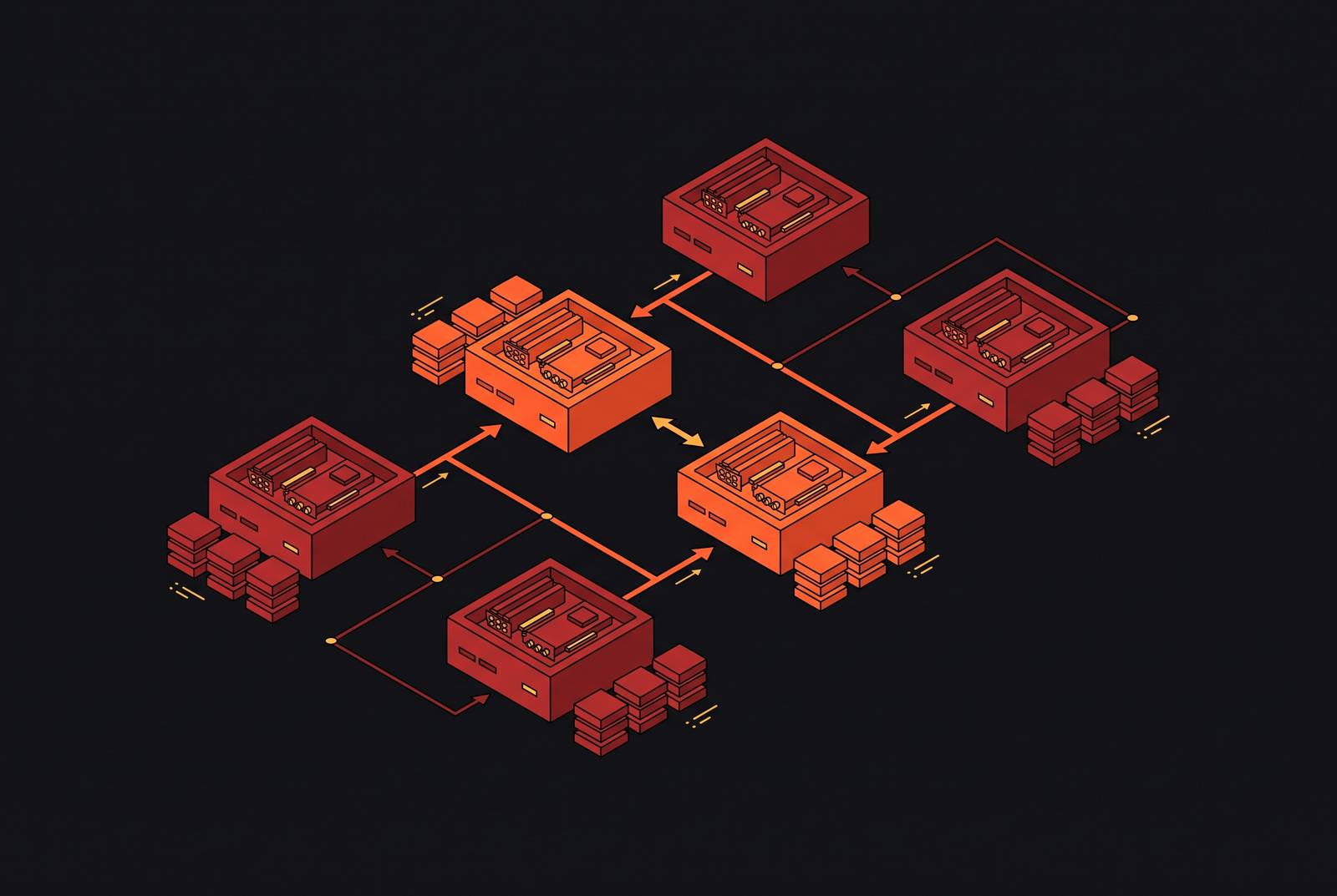
Multi-node training leaves GPUs idle when training samples, activations, and gradients cannot reach the compute that needs them fast enough. To improve utilization, data locality must be built into the storage and memory hierarchy. Faster GPUs and wider interconnects can help, but neither fixes a system that keeps data in the wrong tier or moves it through an inefficient path.

Why multi-node training leaves GPUs idle most of the time

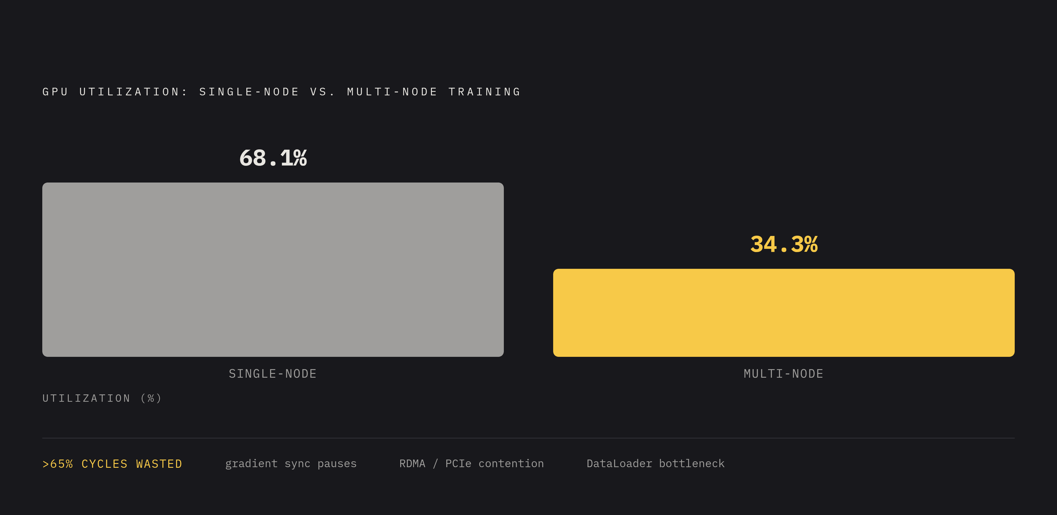
Single-node jobs already lose a lot of GPU time to waiting, and jobs lose even more when they cross the node boundary. The scaling study in the brief found that GPU cycles utilized fell to just 34.3% for jobs that ran across multiple servers. Those servers must stop from time to time to synchronize model state over the network. When jobs compete for shared RDMA and PCIe resources, the wait gets longer, so network bandwidth explains only part of the slowdown.

Default PyTorch DataLoader configurations leave GPUs waiting on CPU preprocessing, which limits how quickly training samples reach compute. That pipeline draws on a six-level memory hierarchy, from registers to NVMe, with speeds that differ by orders of magnitude between the fastest and slowest tiers. The structural gap is between how quickly a GPU can consume data and how quickly the system can deliver it. Adding compute without changing that delivery path leaves the underlying constraint intact.

How the memory hierarchy determines where data lives and how fast it moves

Data residency is the tier that holds a piece of data when compute needs it. GPU HBM provides close access but limited capacity, while host DRAM and NVMe provide other places to hold state at the cost of a longer path. With remote storage, data must also cross the network on that path. These tiers are therefore not interchangeable pools of capacity, even when each can hold the same data.

Within a node, NVLink lets GPUs share memory at up to 1.8 TB/s on Blackwell, making frequent exchanges for tensor parallelism practical. PCIe connects GPUs to host DRAM and NVMe, but PCIe Gen5 can become a bottleneck before any network hop is added. FSDP and DeepSpeed ZeRO use sharding to spread weights, gradients, and optimizer states across GPU HBM. When that distributed capacity is still insufficient, state can spill to NVMe.

Xinnor's offloading benchmark found a large penalty for placing optimizer states on NVMe, with disproportionate overhead for smaller models. The additional capacity solves a fit problem without necessarily solving a throughput problem. Choosing tiers for activations, checkpoints, and model state is therefore an engineering decision that depends on both how much a tier can hold and how long access takes.

Why the training memory footprint is larger than most GPU estimates account for

Weights require 2 bytes per parameter in FP16/BF16, so a large model consumes many tens of gigabytes before training's other demands enter the calculation. Gradients and optimizer states add to that footprint. Activations take up more or less space depending on sequence length and can take up as much as model state at long context windows. A weight-only estimate therefore understates both the capacity required and the volume of data that must remain accessible during execution.

A large frontier model needs a large number of GPUs just to fit, before batch size or throughput determines how many GPUs to use. Teams that omit optimizer states can encounter OOM errors mid-run. That failure shows that capacity to hold weights can fall short of capacity to support the full working set of training. The relevant estimate is the latter.

FSDP is the standard response because it shards weights, gradients, and optimizer states across available GPUs. Accessing state distributed across devices by sharding makes inter-GPU communication a new constraint. Planning must therefore account for both how many GPUs provide enough memory and how the chosen execution strategy moves data between them.

How parallelism strategy determines where data must travel between GPUs

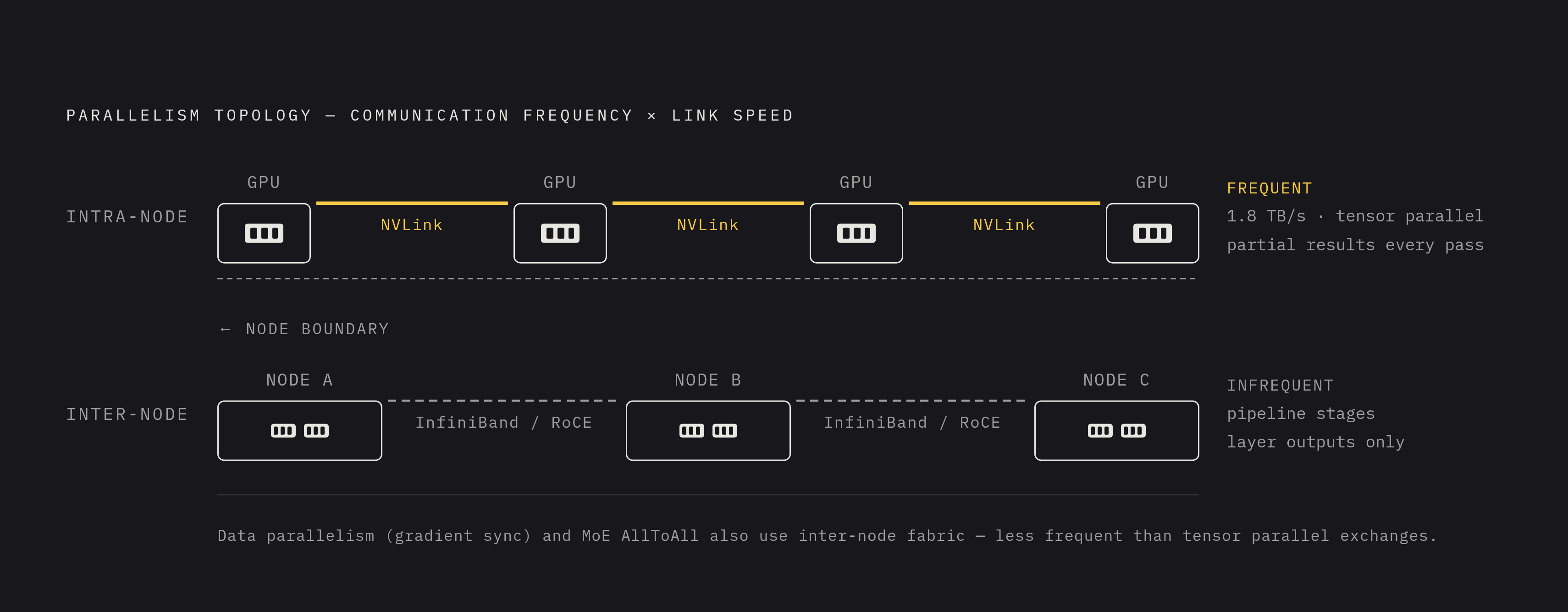
Tensor parallelism splits individual layers across GPUs, requiring exchanges of partial results during every forward and backward pass. Because these exchanges happen so often, they need high bandwidth and low latency. That pattern fits the fast links within a node much better than the slower links between nodes. Tensor parallelism across nodes is therefore usually impractical even when enough aggregate GPU memory is available.

Pipeline parallelism instead splits the model by layers across nodes and passes outputs from one stage to the next. It requires less communication than tensor parallelism, but introduces “bubbles” while a stage waits for the previous stage's output. Modern frameworks combine tensor parallelism within a node and pipeline parallelism across nodes because this arrangement matches communication frequency to the hierarchy.

Data parallelism creates another pattern, scaling well until gradient synchronization saturates the interconnect. MoE models add AllToAll operations that route tokens to expert GPUs and are especially sensitive to inter-node latency. For most teams, the practical starting point is tensor parallelism over NVLink within nodes and pipeline parallelism over InfiniBand or high-end RoCE between nodes. Departures from that pattern require careful measurement.

Whether InfiniBand actually solves the inter-node locality problem better than high-speed Ethernet

InfiniBand has the greatest edge when training needs frequent collective operations across nodes. Low-latency RDMA fabric matters for AllReduce-heavy training and for the AllToAll traffic of MoE models. Other workloads move different data at different rates, so this advantage gives only some workloads a reason to require InfiniBand. The choice of fabric depends on how the workload communicates as well as the size of the cluster.

WWT's MLPerf tests found Ethernet completing BERT-Large training faster than InfiniBand. The same tests found InfiniBand's advantage on LLaMA2 inference was under two percent. Those results show that a workload-specific comparison can differ from the conventional ranking of fabrics.

Crusoe's MLPerf Inference v6.1 result in September 2026 achieved linear scaling across 512 AMD MI355X GPUs coordinated entirely over 400 Gb Ethernet. Crucially, that workload used no cross-node all-reduce. Inference replicas that never synchronize gradients do not impose the same network demands as tightly coupled training. Cluster procurement should therefore match the fabric to collective frequency and communication structure, rather than treating the network label as a proxy for utilization.

Why GPU Direct Storage changes the checkpoint and activation I/O bottleneck

A 140 GB checkpoint can move roughly 280 GB of data through CPU memory in total along the standard five-hop I/O path. The CPU copies data it will never compute on, which doubles memory traffic and adds a hidden cost to GPU time when checkpoints are saved. That CPU-staged path can stall GPUs for minutes per checkpoint. GPU Direct Storage makes the important change to the I/O path by removing the bounce buffer and letting the GPU's DMA engine write directly to NVMe.

Micron's FMS 2026 demonstration showed large-scale random IOPS from a single server across dozens of high-density PCIe Gen6 SSDs. That transaction pattern matters for embeddings, vector retrieval, and KV-cache lookups. The demonstration shows that a well-designed I/O path can keep NVMe performance from holding the system back. Provisioning fast SSDs without addressing CPU staging leaves a separate bottleneck in place.

NVMe over Fabrics extends the direct-access principle across nodes. NVMe/RoCE over 100GbE lets GPUs read from remote NVMe drives without CPU intervention, making networked flash a deliberate tier in the hierarchy. GDS, direct DMA paths, and NVMe/oF therefore belong in the same design discussion as parallelism and interconnects. This matters even more when inference needs to fetch the same state again and again.

KV cache as the inference-time version of the training data locality problem

The KV cache stores intermediate key and value vectors from previous tokens so generation does not repeat that computation. Caching changes quadratic sequence-length complexity to linear complexity, but takes up a large and growing amount of memory. The cache grows linearly with context length and must stay close enough to compute to keep generation from stalling. It is the inference counterpart of training's activation and model-state residency problem.

At very long context lengths, a mid-sized model's KV cache can reach tens of gigabytes and exceed a typical GPU's HBM capacity. Spill to DRAM or NVMe then becomes a normal condition of long-context serving. Changes to the architecture can shrink the footprint before it reaches storage. With Multi-Query Attention, all attention heads share keys and values. Grouped-Query Attention shares them within groups. DeepSeek's Multi-Head Latent Attention re-parameterizes them as low-rank projections.

H2O, Scissorhands, and RoCo use attention scores to identify and drop unimportant KV pairs, while PagedAttention and vLLM use OS-inspired paging to achieve near-zero space waste from fragmentation. These methods defer the capacity problem without eliminating locality constraints at scale. NVIDIA's ICMSP makes the structural response explicit by treating NVMe as a first-class tier of the KV cache address space, making flash a managed home for state.

How prefill-decode disaggregation reorganizes the inference compute and memory topology

Co-located prefill and decode are inefficient because the phases have different resource profiles. Prefill is compute-bound and benefits from fast HBM access, while decode is memory-bandwidth-bound and depends on access to KV state. Running both on the same GPU also increases HBM pressure because that state must be managed for both phases simultaneously. Separating them lets compute placement reflect those different needs.

The disaggregated model uses dedicated prefill and decode worker pools, with a transport layer moving KV tensors between them over NVLink or InfiniBand. NVIDIA Dynamo implements this arrangement as an open-source distributed inference framework above vLLM. Its NIXL transport layer handles KV tensor movement between workers. NVIDIA's headline result is a 30x increase in served requests for DeepSeek R1 on GB200 NVL72 with disaggregated FP4 serving.

The separation still requires protocol-level coordination. Prefill and decode workers compute KV block sizes independently, but those sizes must match for cache transfer. A transport link alone cannot resolve a mismatch in how the workers organize the state being moved. Disaggregation works by placing data in the tier appropriate to the compute phase and connecting those placements with purpose-built transport. It makes locality part of the compute topology rather than treating it only as a memory-capacity issue.

What engineering the storage and memory hierarchy actually requires in practice

Within a node, choose FSDP or ZeRO sharding to keep model state in HBM and NVLink-connected GPUs for workloads requiring tensor parallelism. Plan model size and optimizer choice around the real penalty of NVMe offload. At the node boundary, match fabric choice to the communication pattern rather than assuming all distributed jobs have the same needs. On the storage path, deploy GDS to remove checkpoint and activation bounce buffers, extending direct access through NVMe/oF where data must come from remote storage.

For long-context inference, treat KV cache as a managed data tier with explicit transport between prefill and decode workers. Include NVMe-resident persistent KV state where that architecture requires it. Scheduling must also account for more than current resource availability. TORTA's reinforcement-learning scheduler demonstrates how a spatiotemporal approach can capture long-term workload patterns and short-term execution constraints to reduce inference latency and operational cost.

For MIG deployments serving many smaller models, optimize workload placement across GPU partitions. IBM Research's MIG placement study found that optimization and heuristic methods outperform baseline schedulers on GPU count and utilization waste. These decisions span capacity, transport, and scheduling because an untreated tier can become the next bottleneck. Their common purpose is to move data closer to compute or schedule compute where its data already lives. Proximity is the design variable that controls utilization, and it is engineered.