Unit Cost Curves as LLM Inference Scales From 10 to 10,000 GPUs

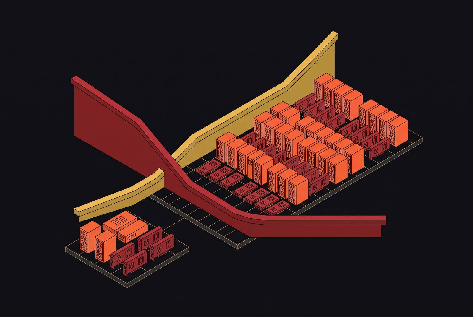
The assumption built into most capacity planning for LLM inference is that cost-per-token falls as GPU count rises, on something close to a straight line. Double the fleet, halve the unit cost. That model breaks down because the binding constraint on cost does not relax evenly as a fleet grows. It changes category entirely at different points in scale, which makes the real cost curve piecewise rather than continuous. If you double the GPU count, cost-per-token does not halve, because what it tracks is utilization and scheduling discipline, far more than raw hardware count. A fleet that is poorly scheduled at ten GPUs stays poorly scheduled at a hundred, and the inefficiency scales right along with it.

Cast AI's 2026 State of Kubernetes Optimization Report checked production Kubernetes fleets and found average GPU utilization at 5%, and the best-performing cluster in that dataset, a large H200 deployment, still came in well short of half utilization. A fleet near zero utilization pays full hardware cost for every idle card, so when you scale it tenfold, you multiply the idle spend, not the useful throughput. Moving to a newer GPU generation does not fix this arithmetic on its own, since price climbs faster up the stack than throughput does, and the same optimization failure that wastes money at a small GPU count scales proportionally to a very large one.

What changes as a fleet scales is which constraint binds the cost curve. At small scale, what limits you is memory capacity and how fully each card gets used. In the mid-range, the limit becomes the architecture of KV cache storage and the discipline of the batch scheduler. At the largest deployments, the limit shifts again, to interconnect topology and storage I/O throughput. Each regime has its own highest-leverage fix, and applying the fix for one regime to a fleet operating in another regime tends to produce little return, because the lever that mattered at the last scale is no longer the one holding cost in place.

Regime one (tens of GPUs): memory capacity and utilization per card as the primary cost lever

At the scale of tens of GPUs, cost-per-token is set mostly by whether a model fits in the memory available and how much of that memory does useful work between requests. A model that needs tensor parallelism across two cards pays a communication tax that a single-card deployment never incurs. A large frontier model at BF16 precision needs well over a hundred gigabytes of weights, before you even count KV cache or activations, so an H100's 80 GB forces that model onto two cards, and that doubles the hardware footprint and adds NVLink synchronization overhead on top. Precision format is the first cost lever available at this scale. FP8 halves the weight memory a model needs, and because the B200 carries 180 to 192 GB of HBM3e, a model that would otherwise need two H100s (a combined 160 GB) can run on a single B200 instead. The H200's 141 GB of HBM3e produces the same kind of gain: it lets large models run on one card where two H100s were previously required, and that single-card configuration is reported to bring substantially lower per-token costs.

The second lever is idle time. GPU time-slicing and MIG partitioning both let one physical card serve more than one workload at once. On an 80 GB A100, MIG profiles range from a small slice that fits a quantized small model up to the full card, which a large BF16 model needs in its entirety. MIG's isolation is strict enough that NVLink and peer-to-peer CUDA communication are switched off between partitions, so tensor parallelism across two MIG slices on the same card is not possible, and MIG only helps for models that already fit inside a single partition. Time-slicing works differently and more broadly. It runs on any CUDA-capable NVIDIA GPU, including older cards like the T4 and A10G as well as Ampere and later generations, and it multiplexes access at the scheduling level rather than through hardware isolation. That has a cost: without memory isolation, noisy-neighbor effects occur in shared scheduling, which makes time-slicing a poor fit for latency-sensitive production traffic.

Batching is the single change at this scale that moves cost the most without adding any hardware. If you shift from single-stream serving to continuous batching, even at modest batch sizes, you can cut cost-per-token by a large multiple. That gain has a boundary, though: it holds at shorter context lengths, and once context grows, the KV cache starts competing with model weights for the same memory, which caps how large a batch the card can actually sustain.

Poor scheduling and utilization decisions compound silently at this scale: a request's token-normalized cost can look better even as its total energy spend goes up. A CMU energy characterization study running on H100 and H200 hardware found that, for a small model at a moderate batch and context size, lengthening the output reduces the energy cost per token substantially, while the total energy spent across the batched inference window actually rises. That happens because a longer output spreads a fixed prefill cost across more generated tokens. So the joules-per-token figure improves, but the GPU is not using less energy overall. An operator optimizing only for cost-per-token at this scale can end up raising total energy spend and infrastructure cost at the same time. The actual target needs to be request energy and token energy considered together, not one in isolation.

Regime two (hundreds of GPUs): KV cache architecture and batching discipline as the controlling variables

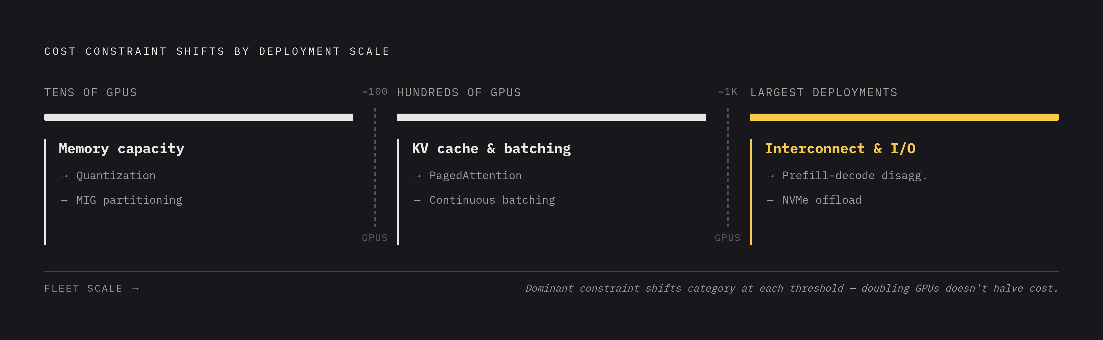
Once a fleet reaches hundreds of GPUs, raw memory capacity per card stops being the whole story. The architecture used to store and manage the KV cache, along with how sophisticated the batch scheduler is, takes over as the main driver of cost-per-token.

The inefficiency that traditional inference systems never solved is fragmentation. Without a paged memory scheme, KV cache fragmentation wastes most of the memory allocated to it. vLLM's PagedAttention treats the KV cache the way an operating system treats virtual memory, splitting it into non-contiguous blocks, and that cuts fragmentation waste to under 4% while producing throughput gains of two to four times. Continuous batching adds to that gain on its own terms: a new request joins the batch the moment a slot frees up, instead of waiting for the whole batch to finish, and that alone produces two to four times higher throughput at the same hardware budget.

At mid-range context lengths, KV cache memory starts to rival or exceed the memory the model's own weights take up, and that is the physical cause of the inflection point this regime represents. A large model running at long context can need tens of gigabytes of KV cache for a single request, and a sizeable batch multiplies that into hundreds of gigabytes, well past what one node's HBM can hold. FP8 KV cache halves the per-token memory footprint compared to BF16, but even with that gain, you can still see KV cache alone consume more than half of a single H100's 80 GB for a large model at very long context, before its weights are even loaded.

Prefix caching and speculative decoding act as secondary levers on top of PagedAttention that compound its gains. Prefix caching reuses the KV cache for prompt prefixes that repeat across requests, which covers a lot of real traffic: chat sessions, RAG pipelines with a fixed system prompt, and agentic loops that reuse context turn after turn, all of which see substantial drops in time-to-first-token on a cache hit. Speculative decoding works differently. A small draft model proposes several tokens ahead, and the main model verifies them in a single forward pass, so you get its biggest latency gains at low concurrency for chat and copilot-style workloads. Cast AI's guide is direct about the limit here: the benefit shrinks as concurrency and batch size grow, so the only reliable way to know whether it helps a given deployment is to measure it at the concurrency that deployment actually runs.

Sizing a fleet at this scale by simple arithmetic does not work, because queuing behavior under heavy-tailed workloads defeats the kind of back-of-envelope reasoning that works at smaller scale. A March 2026 simulation tool called inference-fleet-sim combines M/G/c queuing theory with discrete-event simulation, so it can find the cheapest fleet configuration that still meets a time-to-first-token service level. Its seven case studies each surface a result that simple analysis gets wrong: a fleet that looks underutilized still fails its latency target, a slower GPU beats a faster one on cost, GPU scaling turns out to be sub-linear, and the router used to size the fleet in simulation is not the router that runs in production. The sub-linear finding carries the most weight for this regime: adding GPUs without also fixing routing and scheduling can produce diminishing, even negative, returns on cost-per-token.

The prefill/decode disaggregation architecture addresses the mid-range bottleneck structurally by separating the compute-intensive prefill phase from the memory-bandwidth-intensive decode phase. Moonshot AI's Mooncake architecture, presented at USENIX FAST 2025, builds on exactly that separation, and describes its own approach as trading more storage for less computation: KV cache gets routed across network storage tiers instead of being recomputed, which lets prefill pools and decode pools scale independently of each other. Once KV cache starts moving off the GPU entirely, storage I/O throughput becomes a cost variable in its own right, not merely a tuning detail.

KV cache as a physical storage problem

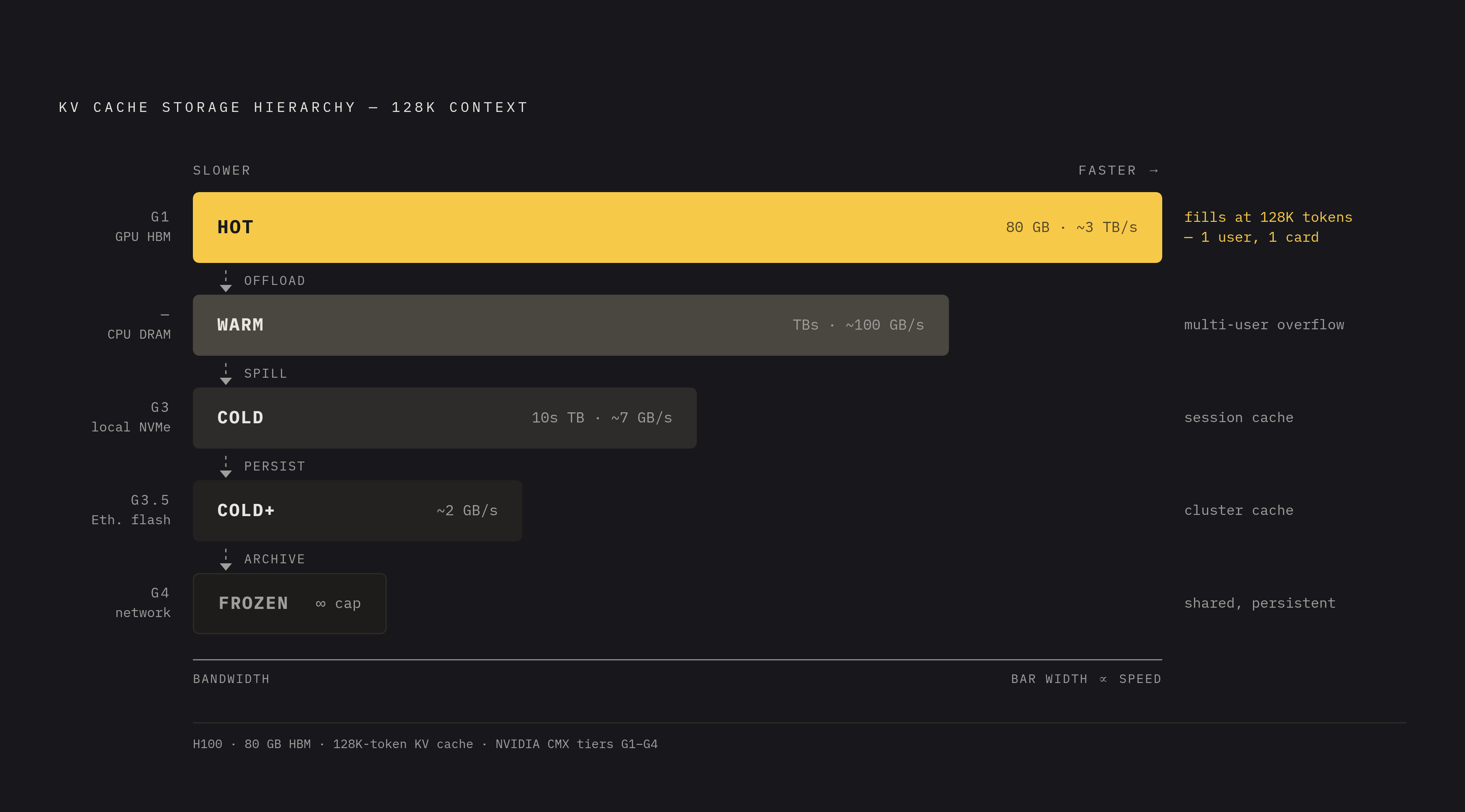
At the context lengths production systems now handle routinely, a scheduler can no longer manage KV cache inside GPU memory. It becomes a storage architecture question, and that question decides whether serving long context is economically possible at all.

The constraint is physical. At 128K tokens of context, a single H100 cannot serve more than one concurrent user without offloading KV cache somewhere else. A single user's KV cache at that context length already takes up a large share of the card's HBM, and a handful of concurrent users would need several times the H100's entire memory, so the only way to serve them on one card is to move cold KV blocks off the GPU. No batching trick or quantization scheme removes this limit. FP8 KV cache halves the memory each user needs and shifts how many users can share a node, but it does not change the underlying constraint.

The production answer to that constraint is a four-tier offload hierarchy: hot cache is held in VRAM, warm cache in CPU DRAM, cold cache on local NVMe, and shared or persistent cache in network storage. Cache-aware serving is what makes that hierarchy economically workable, because it routes a given request to whichever node already holds the relevant KV blocks. The traffic patterns that benefit most are the ones with repeated context: multi-turn chat, RAG pipelines with a repeated system prompt, and agentic loops that carry long shared context across steps, all of which see large reported improvements in time-to-first-token when a request lands on a node with a cache hit.

NVIDIA's CMX, announced at CES 2026, extends GPU KV cache into NVMe storage through a five-tier hierarchy: G1 is GPU HBM, G3 is local NVMe, G3.5 is Ethernet-attached flash, and G4 is network storage. The design treats NVMe-resident KV cache as part of the context memory address space, so it persists across separate inference runs and does not disappear when a session ends. NVIDIA claims its own figures show up to five times the power efficiency of traditional storage and up to five times the tokens-per-second. The serving framework built to use this hierarchy, Dynamo, works across GPU HBM, CPU DRAM, direct-attached NVMe SSDs, and networked external storage, using Spectrum-X Ethernet or InfiniBand and RoCE for RDMA-based access.

Whether offloading to NVMe actually beats recomputing prefill is not a settled question, and it inverts depending on where a deployment sits. At the context lengths now common in production, storing and reloading KV cache from NVMe is usually faster and cheaper than recomputing prefill from scratch. But that conclusion flips at short context lengths or under a high cache-miss rate, where even Gen5 NVMe's read latency becomes the bottleneck instead of the fix. The break-even point depends on the ratio between prefill compute cost and NVMe read latency for the specific model, context length, and cache hit rate in question, so you need a measured baseline for your own workload, not a rule carried over from somewhere else.

One more gain stacks on top of quantization rather than replacing it. Intel research found that for FP8 formats, the exponent values keep enough statistical skew to compress well, with the compressed exponent taking up only a small fraction of its original size, while the mantissa stream compresses less readily. KV cache tensors show the same exponent skew that model weights show. This compression produces real memory savings on cold KV blocks sitting in the lower tiers of the storage hierarchy, on top of whatever quantization has already achieved.