MLPerf Training Benchmarks as Infrastructure Scaling Indicators

MLPerf Training measures how long it takes a fixed model to reach a defined quality target, under audited conditions that every submitter has to follow the same way. The result is a full-system benchmark, not a chip test, and reading it as infrastructure signal rather than a hardware leaderboard is the subject of this piece.

What MLPerf Training Measures

MLPerf Training is built and run by MLCommons, an open engineering consortium that brings together academia, industry, and civil society. Results go through peer review and come out on a cadence of roughly every six months, giving the field a running record of how fast the infrastructure underneath AI training is actually moving, since that cadence tracks deployed systems rather than chip announcements.

The suite splits into two divisions. The closed division requires submitters to use a reference model, so everyone trains the same architecture to the same quality bar and differences in time-to-train trace back to the system underneath it rather than to a different model someone chose to run. The open division allows more latitude in model choice and is useful for other purposes, but it's the closed division that carries the infrastructure signal this piece is built around, precisely because its software constraints are standardized across every submitter.

What makes time-to-train a useful diagnostic is that the clock doesn't stop at the GPU. If a system has fast GPUs but its storage layer can't feed them fast enough, it still posts a slow time. That single design choice, measuring the whole pipeline instead of isolating the processor, turns MLPerf Training into something infrastructure engineers can read for bottlenecks.

How v5.0 and v6.0 changed what the benchmark tests

The benchmark suite doesn't stand still, and the changes between v5.0 and v6.0 show MLCommons tracking the architectures that actually run in production. v5.0 set a record with more than 200 total submissions, and most of the individual benchmark tests carried over from v4.1 saw submission counts rise, a sign of a benchmark that organizations were investing more effort into each round.

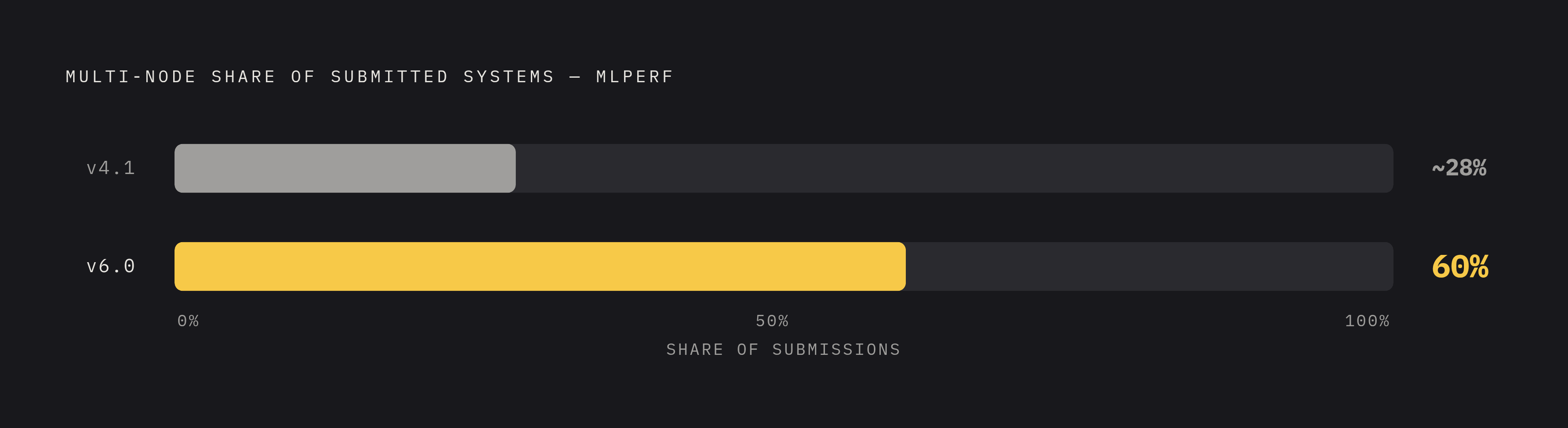
v6.0, published June 16, 2026, took a sharper turn. DeepSeek V3 is now the largest workload the suite has ever included. MLCommons reports that v6.0 drew submissions from numerous organizations running dozens of unique systems, and that participation in multi-node configurations rose substantially compared to v4.1, with 60% of v6.0 systems running multi-node versus a far lower share in the earlier round.

The two new workloads were scoped deliberately at opposite ends of the infrastructure spectrum. DeepSeek V3 needs large multi-node clusters, so it pushes submitters toward them almost by necessity. That means v6.0 tests both ends of the infrastructure scale at once, from a single node's local memory and storage behavior up through thousands of GPUs coordinating over a shared fabric.

v6.0 also marked the first appearance of vendor-specific FP4 formats in submitted results. That detail matters beyond the numbers it produced: it tells infrastructure teams that lower-precision training has matured enough to survive an audited, peer-reviewed benchmark process, not just a vendor's internal testing.

How Adding DeepSeek V3 as a Benchmark Workload Changes the Infrastructure Signal

Dense transformer benchmarks, the kind that dominated earlier MLPerf rounds, stress GPU compute and memory bandwidth in ways that are comparatively easy to isolate. Mixture-of-experts workloads break that pattern. They stress storage random-read IOPS, interconnect routing, and memory capacity all at once, so the infrastructure bottleneck appears directly in the final score.

DeepSeek V3 activates only a small fraction of its 671 billion parameters for any given token. That sparsity drives a fine-grained, sparse I/O pattern across a weight tensor far larger than what any current GPU's on-board memory can hold, and that tensor has to stay reachable at low latency no matter which expert a given token needs.

One vendor's own submission illustrates how immediately this forces a shift in system design: the company scaled to thousands of GPUs using a high-interconnect multi-GPU rack-scale system for its DeepSeek V3 submission, the largest-scale submission of its kind MLPerf Training has seen to date. It forces multi-node, high-interconnect configurations from the start, which is exactly where storage and fabric performance become the limiting factor.

GPT-OSS plays a different but complementary role. Because it's scoped to a single 8-GPU node, it lets infrastructure teams isolate per-node memory hierarchy and local NVMe performance without the confounding effects of a multi-node interconnect. Between the two workloads, v6.0 gives infrastructure engineers a cleaner separation of variables than any prior round: one workload for diagnosing a single node's internal architecture, and one that makes cluster-scale fabric and storage performance impossible to hide from.

Reading time-to-train scores as infrastructure diagnostics rather than chip rankings

The raw time-to-train figure in a results table looks like a single number, but it's a composite of several different systems working together, and the diagnostic value comes from comparing how that number changes across node counts, precision formats, and workload types.

Look first at scaling behavior as node count increases. The rate of that slowdown is the signal worth tracking, not the absolute time posted at any single node count.

Look next at how a system performs across workload types. A system that does well on compute-dense benchmarks but falls behind on MoE workloads relative to its node count is running into a memory-capacity or random-read IOPS ceiling. That gap appears because expert weights have to stay reachable even when they aren't currently active in HBM, and a system that can't serve that access pattern efficiently will post a worse MoE score than its dense-model results would predict.

Software maturity leaves its own trace in the version-over-version data. v5.0 results showed the Stable Diffusion benchmark improving at more than twice the rate Moore's Law would predict for 8-processor systems, and more than three times that rate on 64-processor multi-node configurations. Hardware generation turnover alone cannot produce gains that size. So the improvement points to better collective communication and data-pipeline tuning in the software stack itself.

You can check checkpoint overhead directly against the tables too. At the scale of large MoE models, each checkpoint write demands a large sequential write against shared storage. A system whose time-to-train includes a heavy checkpoint tax relative to peers running the same node count is storage-bandwidth-constrained, and that constraint adds measurable time even if the system's raw compute throughput looks competitive.

Submissions have to alternate between training and evaluation at short intervals once they reach large scale, which imposes a context-switching overhead that production training jobs don't usually face.

Storage as the infrastructure layer that time-to-train most reliably exposes

Because the benchmark clock runs across the whole system, storage bandwidth and IOPS print directly into the final time-to-train result. That makes MLPerf one of the few audited, peer-reviewed venues where storage infrastructure quality gets tested competitively instead of staying an internal engineering detail nobody outside the organization ever sees.

The mechanism is simple to state and expensive to ignore: when storage throughput falls short, the data pipeline stalls, and GPUs sit idle waiting on the next batch. The most expensive resource in the system ends up waiting on the cheapest one. MoE workloads make this worse. Sparse expert routing means storage has to serve fine-grained, non-sequential reads against a weight file far larger than anything that fits in GPU HBM, so it puts far more pressure on random-read IOPS than dense-model training ever did.

Checkpointing adds a second, separate kind of storage stress. Systems that write checkpoints asynchronously to node-local NVMe, rather than synchronously to a centralized store, can cut the bandwidth demand on shared storage by a substantial margin, and that difference appears directly in time-to-train at scale.

Parallel file systems built on NVMe-over-Fabrics give a shared storage tier a way to approach local-NVMe latency while still handling concurrent access from thousands of GPUs at once. That architectural choice is one of the clearest dividing lines between high-efficiency and lower-efficiency MLPerf submissions running the same node count. The same tiered logic that governs inference-time memory hierarchies, moving data between GPU HBM, host DRAM, and NVMe as needed, applies on the training side too: pre-staging data on fast local NVMe ahead of time removes the centralized storage system as a chokepoint before training ever starts.

Interconnect as the multi-node scaling constraint that MoE workloads make visible

When a job crosses a node boundary, DeepSeek V3-scale MoE training makes the interconnect fabric the dominant variable in the result.

Dense transformer training mostly stresses point-to-point gradient synchronization between nodes, and collective-communication libraries have been tuned against this pattern for years. MoE adds something harder: irregular all-to-all routing of activated expert inputs across the cluster, sensitive to both bandwidth and latency in ways that require collective-communication software to be tuned specifically for this routing pattern. CCL-Bench, a trace-based benchmark built specifically for LLM infrastructure, covers compute, memory, and collective communication together, and its existence is itself evidence that large-LLM communication patterns are distinct enough from earlier workloads to need dedicated measurement. MLPerf's multi-node scaling results can confirm that this distinction matters in practice, but the benchmark alone can't fully decompose which part of the fabric causes a given slowdown.

The choice between RoCE and InfiniBand carries real operational weight at this scale, and the sources don't resolve it one way. Neither option wins outright at every scale, so submitters have to trade configuration burden against raw performance ceiling.

That tradeoff gives readers a concrete way to interpret the multi-node results tables: a submission using RoCE that achieves near-linear scaling as node count rises is demonstrating fabric engineering maturity, not just raw hardware generation. A system that scales well in an MLPerf submission isn't guaranteed to hold that same scaling curve in a production cluster carrying other traffic at the same time.

Storage and interconnect concerns meet directly at NVMe-over-Fabrics using RDMA. The latency profile of this path, which avoids the SCSI emulation layers that older storage protocols rely on, is what lets parallel file systems sustain the throughput that large-scale training jobs demand from a shared storage tier serving thousands of GPUs at once.

How precision format choice determines which memory tier binds

For an infrastructure engineer, choosing a numerical precision format is a decision about which memory tier weights, gradients, and activations will live in: GPU HBM, host DRAM, or NVMe-backed storage reached only through an offload path.

FP8 cuts the memory footprint per parameter in half compared to BF16. That difference can decide whether a large model fits entirely inside the HBM on a given system configuration or instead needs weight movement between nodes, and at scale it compounds into a measurable gap in training throughput.

MoE models complicate this further, and asymmetrically. The expert weights active for a given token fit comfortably into HBM at FP8 precision. That fact makes the storage and interconnect layers structurally necessary parts of the system rather than optional performance add-ons, since no precision trick alone makes the full model fit on-chip.

So if you're an infrastructure engineer reading v6.0 results, treat those FP4 numbers as an early marker of which memory hierarchy constraints the next generation of hardware is being designed to relieve.

Compression research adds another lever to this same problem. BF16 tensors, once normalized, tend to show a narrow and skewed distribution in their exponent field, a pattern that gets more pronounced after normalization. Lossless compression that exploits this pattern has shown real results: one documented approach, TRACE, achieves a 46.9% reduction in BF16 KV cache footprint and a 25.2% reduction in weight footprint, both without any loss of precision. That kind of reduction cuts the bandwidth needed to move weights and cache entries between memory tiers, and the same principle applies directly to training checkpoint I/O and weight staging, not just to inference.

So a storage layer has to handle multiple precision formats inside the same checkpoint without corruption or added alignment overhead, which is one more reason you can't treat precision format choice and storage architecture as separate decisions.

KV cache memory pressure as the inference-side analog to the training storage problem

The same memory-tiering pressure that shapes training storage architecture reappears on the inference side, in the form of KV cache management. During inference, each token generated adds to a growing cache of key-value pairs that has to stay reachable for the length of a session, and that cache competes for the same GPU HBM that model weights occupy. The documented response in the literature is a hybrid memory hierarchy: moving cache data between GPU HBM, host DRAM, and NVMe SSDs as a session's memory needs grow beyond what fits on-chip. The 46.9% reduction in BF16 KV cache footprint that TRACE demonstrates speaks directly to this problem, cutting the volume of data that has to move between tiers. Training and inference end up facing a version of the same constraint from opposite directions: training must move enormous weight tensors to where compute happens, and inference must keep a growing cache reachable without crowding out the weights already resident in HBM. Both problems point back to the same underlying architecture question that the storage and interconnect sections above lay out: how fast and how cheaply data can move between memory tiers, under real production load, once a model outgrows what GPU memory alone can hold.