What vLLM, TGI, and SGLang Benchmark Results Actually Tell You About Production Storage Requirements
Benchmark rankings hide the storage architecture each engine demands.

Open-source LLM inference stack benchmarking and optimization requires reading throughput, latency, and GPU utilization as storage specifications as well as engine rankings. vLLM, TGI, and SGLang expose different KV cache architectures through their results. Reproducing those results in production depends on matching the benchmark’s cache capacity, bandwidth, locality, and precision conditions.
Why benchmark numbers for vLLM, TGI, and SGLang are really KV cache architecture signatures
A practitioner reading an inference benchmark table usually looks for the engine with the highest throughput or lowest latency. But that ranking hides the conditions that made the result possible. Each engine makes a different bet on where KV data lives and how it moves. The numbers are consequences of those choices.
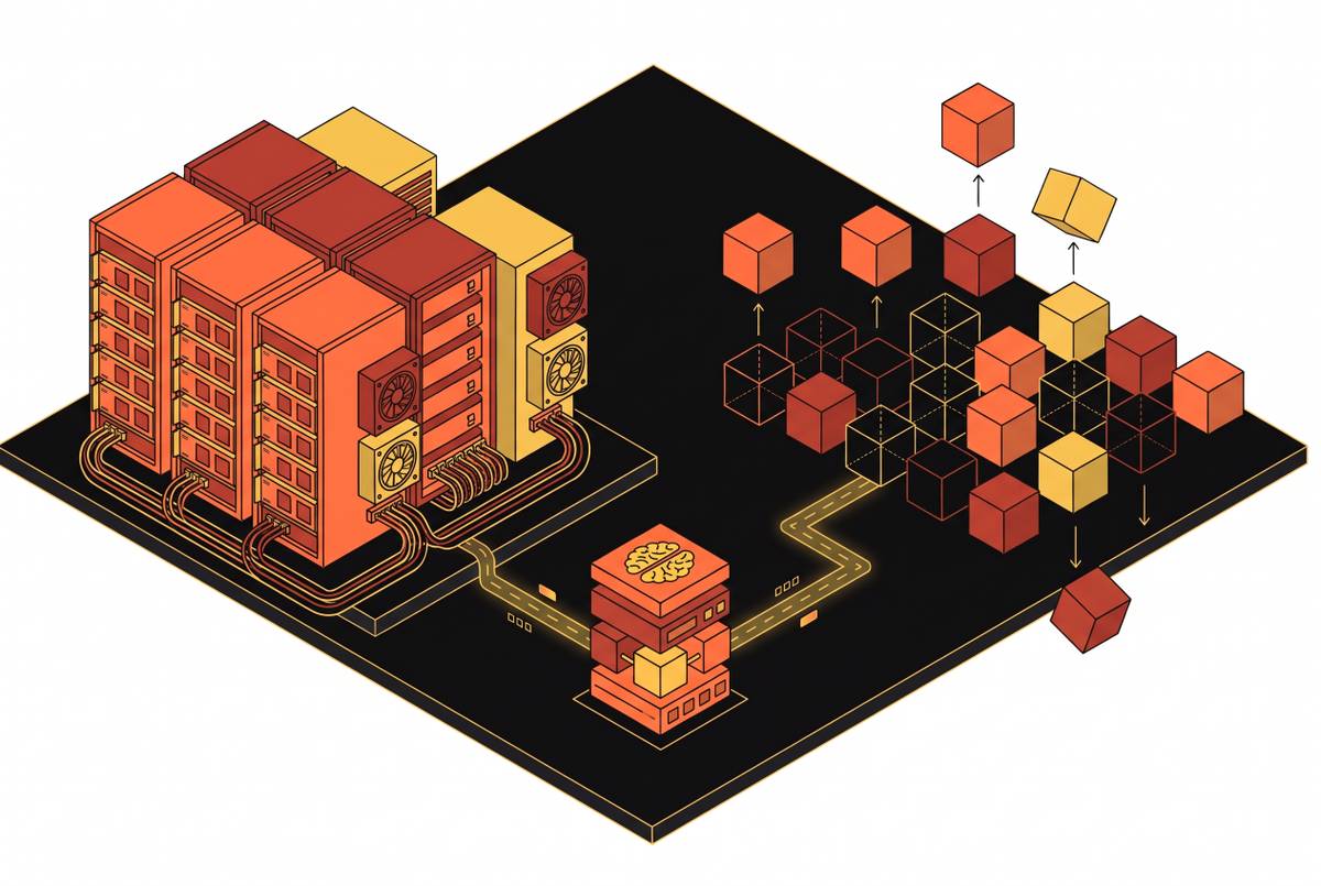
vLLM’s PagedAttention uses fixed-size blocks and OS-style virtual memory to address KV cache fragmentation. SGLang’s RadixAttention uses a prefix-tree cache to reuse KV states across requests with a common prefix. TGI combines continuous batching with native integration into a model-hosting platform but has no equivalent KV reuse mechanism. These differences reach below the engine itself. They place different demands on GPU memory, CPU DRAM, and NVMe storage, which a table for choosing an engine alone does not explain.
How KV cache memory pressure is the structural force behind every benchmark number
KV cache memory grows linearly with context length because key-value data must be stored for every token. For a given model and precision, the per-token footprint is fixed, so longer contexts multiply capacity requirements directly. The scale can exceed a single GPU. At very long context windows, one large Llama 3.1 session can require more KV cache than the combined HBM of multiple H100s. Concurrency puts more pressure on memory because more sessions’ states must stay there at once.
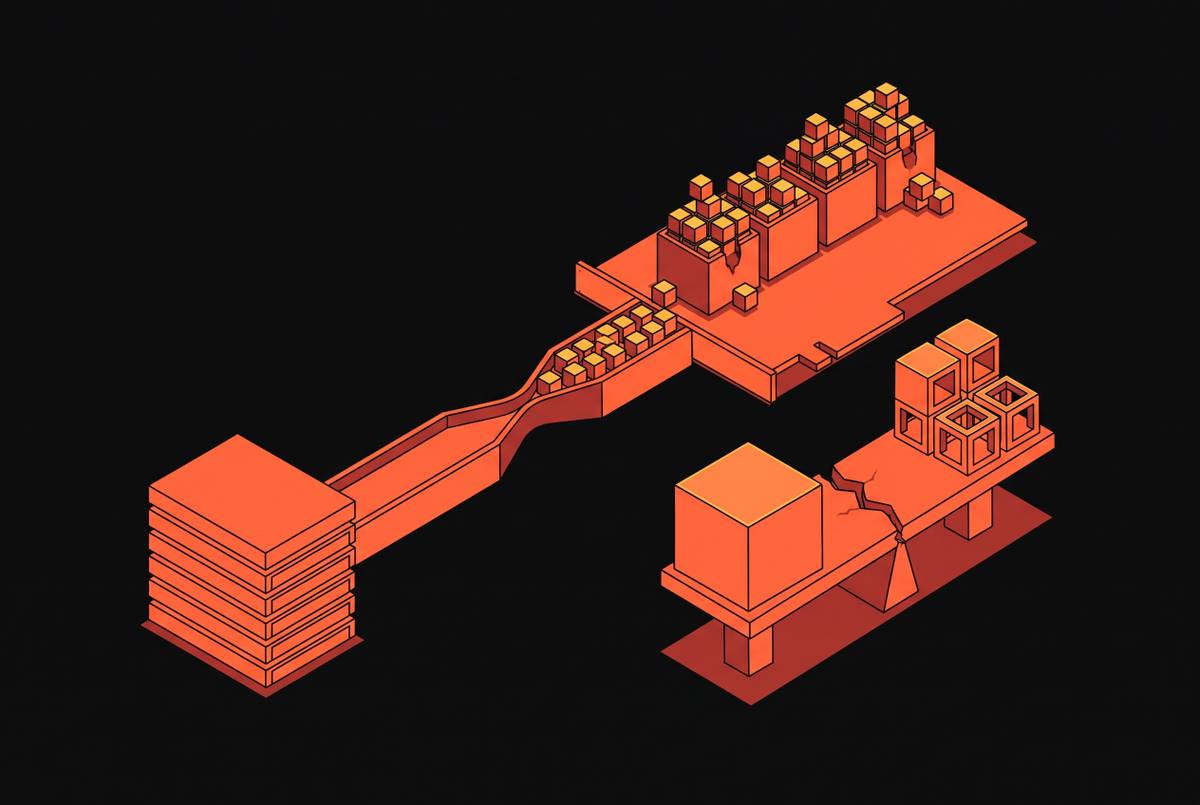
GPU HBM provides roughly 3.35 TB/s, while CPU DRAM reached through PCIe 5.0 provides roughly 64 GB/s, about 2% of HBM bandwidth. Local NVMe accesses take 20–100 µs, with bandwidth orders of magnitude below HBM. Offloading frees memory but adds time to move the data. Recomputing KV states consumes GPU compute, while retaining and reloading them consumes capacity and I/O bandwidth. The engine’s approach to that trade-off shapes the throughput and latency its benchmark reports.
What PagedAttention's efficiency numbers actually encode as storage requirements
PagedAttention’s efficiency numbers describe better use of GPU memory with total KV data unchanged. Traditional engines allocate a contiguous memory block per request and waste 60–80% of KV cache memory through fragmentation. PagedAttention instead places fixed-size blocks wherever space is available, reducing waste to a small fraction. The immediate benefit is larger batch sizes. The storage consequence is that more useful KV data can remain active on the same hardware.
The comparison with TGI at 50 concurrent users on a moderately sized model illustrates this distinction. vLLM consumes significantly less VRAM, creating room for more concurrent sessions while keeping each session’s KV states the same size. Those additional sessions can amplify traffic to the storage layer. On bursty, mixed-length workloads without shared prefixes, continuous batching produces a relatively uniform KV write pattern suited to sequential NVMe provisioning. Reads matter more as more prefix caching is enabled and the cache hit rate in production rises.
The provisioning requirement is sustained write bandwidth, with read bandwidth sized to the amount of cached KV data actually reused.
What RadixAttention's prefix-hit numbers encode as storage requirements
RadixAttention’s advantage comes from its prefix trie retaining KV states that a later request with the same prefix can reuse without recomputation. Cache residency is therefore a performance precondition. In synthetic comparisons with unique prompts and effectively no cache hits, SGLang and vLLM converge to within a few percent of each other. That result locates the observed advantage in prefix reuse rather than a general advantage across all workload shapes.
To keep that advantage, there must be enough fast memory to hold the shared-prefix working set at peak concurrency. Growing contexts, additional sessions, and limited KV capacity all increase eviction pressure. Once useful prefixes leave fast memory, the benchmark’s reuse assumptions break. HBM residency supports the published low-latency behavior, while a spill into DRAM raises time to first token, or TTFT. Spilling the working set to NVMe undermines the hit-rate advantage further, so deploying SGLang with insufficient fast-tier capacity will not reproduce its prefix-heavy benchmark results.
What TGI's maintenance-mode status means for teams reading its benchmark numbers
TGI’s maintenance-mode status changes how teams should use its benchmark results to plan. Its numbers remain useful for teams running it in production, because they describe the behavior of that deployed architecture. They are not interchangeable with requirements for a newer engine. As concurrency grows, the throughput gap against vLLM widens because TGI’s batching does not sustain GPU utilization under load. In that situation, the engine is the binding constraint.
For a team in that position, more storage bandwidth is unlikely to fix the main bottleneck. Migration changes the calculation, however, because vLLM can support more active KV traffic and SGLang can depend more heavily on prefix residency. Teams need to model how much storage the new engine will need before migration. A storage system adequate for TGI does not, by that fact alone, establish readiness for either alternative.
Why the benchmark-to-production performance gap is itself a storage specification
Published benchmarks tend to test conditions one at a time that production must deal with at once. Mixed queues combine prefix-heavy requests with unique prompts, while new sessions begin with cold caches. As the load continues, working sets grow beyond what the fast tier can hold. Evicted blocks must return from SSD, and that reload delay appears in tail latency, with a potentially less pronounced effect on median throughput. The expected 30–50% drop in production performance thus points to storage conditions that the synthetic result leaves out.
The diagnostic sequence should start with cache hit rate under real traffic, eviction rate under sustained concurrency, and SSD reload latency at peak load. Engine version or model quantization should not displace those checks. Each measurement identifies a different failure of the benchmark’s assumptions, including insufficient reuse, insufficient residency, or insufficient reload performance. MLCommons released MLPerf Storage v3.0 results on September 1, 2026, adding a KV Cache test for inference cache read/write operations to the existing training and checkpointing tests.
The three-tier storage hierarchy and what each engine's benchmark signature demands from it
GPU HBM is the first tier, holding hot KV blocks for active generation across all three engines. With roughly 3.35 TB/s of bandwidth, locality makes a decisive difference. PagedAttention increases the share of HBM occupied by useful data rather than fragmented allocations, helping sustain GPU utilization. RadixAttention places an additional demand on that space because shared prefixes must stay resident to deliver its strongest latency results. HBM sizing therefore depends on both active generation and the reusable working set.
CPU DRAM is the second tier, providing a less expensive extension for KV overflow. A node with 8 GPUs can justify 1–2 TB of system memory for that role. But capacity is not equivalent to HBM performance. With roughly 64 GB/s on the PCIe 5.0 path, DRAM is a good fit for semi-warm blocks that are off a low-latency response’s critical path. For vLLM with APC enabled, recently evicted prefix blocks with a reasonable chance of reuse belong in this tier.
NVMe is the third tier, offering roughly 7 GB/s sequential bandwidth and capacity for colder KV states. For very long single-turn RAG workloads, reloading from NVMe can be far faster than recomputation, with the crossover moving earlier as context grows. Continuous KV writes also impose endurance requirements. Datacenter-class drives with high DWPD and multiple drives for bandwidth parallelism are required. Driver behavior must match the transfer size because fine-grained GPU NVMe access paths can leave bandwidth unused when KV reloads need medium-size contiguous transfers.
Tutti, presented at FAST’26 and integrated into vLLM, demonstrates this tier’s potential. It saturates NVMe bandwidth and reduces GPU stalls to near zero, achieving nearly the inference performance of DRAM-backed LMCache with effectively unlimited capacity. Commercial servers with over 100 TB of NVMe can retain more than an hour of KV cache for long-running conversations and agentic workloads. Capacity alone is not the achievement here. The result depends on making that capacity accessible without prolonged GPU stalls.
NVIDIA’s Inference Context Memory Storage Platform, announced at CES 2026 and rebranded CMX at GTC 2026, formalizes the hierarchy in hardware. It offloads cold KV blocks from HBM to NVMe over BlueField-4 DPUs, targeting up to 5x tokens-per-second and substantial power efficiency gains. IBM is working with NVIDIA to combine IBM Storage Scale’s global namespace and locality-aware placement with the platform on NVIDIA Rubin. Both examples connect usable storage capacity to the path through which KV data reaches the GPU.
How FP8 KV quantization and mixed-precision strategies change the storage math
KV precision is a direct capacity and bandwidth variable. Halving precision halves the storage needed for KV data and the I/O required to move it between tiers. In vLLM, turning on --kv-cache-dtype fp8 lets NVMe hold twice as much KV data as BF16 and cuts the bandwidth needed to move it by half. A benchmark measured with FP8 KV cache cannot be translated into a BF16 storage budget without adjusting those quantities.
AMD’s MLPerf Inference v6.1 submission served DeepSeek-R1 through SGLang on 8 AMD Instinct MI355X GPUs. It used MXFP4 for experts and attention output projection, BF16 for the remaining MLA projections, and FP8 for KV cache. The distinctions are essential to interpreting the result. MXFP4 expert weights do not establish the KV storage footprint, because the cache has its own precision. The published throughput belongs to that mixed-precision configuration.
Storage compression and transfer paths must also fit the formats they handle. BF16 and FP8 need strategies built for them to make full use of bandwidth, rather than ones based on systems optimized for FP32 or INT8. Precision alone does not solve transfer granularity. The NVMe driver must still be set up to serve KV blocks efficiently, while compression must keep the storage savings it is meant to deliver. The same MLPerf Storage release adds support for S3 object storage alongside POSIX, so cache read/write performance can be measured through more storage interfaces.
Reading a benchmark table as a storage specification checklist
A benchmark must give six answers before its numbers can be used as a storage specification. Most published tables provide fewer than three. First, a benchmark must specify the model size and KV-per-token footprint at the tested context length. The second is the workload’s prefix overlap and whether it resembles production traffic. The third is the KV precision itself, distinguished from weight and projection precision, because it directly determines cache capacity and transfer volume.
Fourth, a benchmark must specify concurrency, including whether the cache was warm or cold when measurement began. The fifth is the cache’s residency across HBM, DRAM, and NVMe. The sixth is the eviction policy and whether reported latency includes SSD reloads. These are acceptance criteria. Where answers are missing, assumptions must be checked before the result can guide a hardware choice.
The resulting decision rules follow workload shape. Prefix-heavy agents, shared-context RAG, and multi-turn chat call for fast-tier capacity sized to their shared-prefix working set, with HBM residency needed to reproduce the strongest latency results. For unique-prompt, high-concurrency generation and batch processing, NVMe write bandwidth, endurance, and parallel drives matter more. For long-context single-session work, NVMe capacity matters more. Tutti establishes that SSD-backed KV can approach DRAM-backed performance when the transfer path supports it.
Before teams commit to offloading, they still need to check the token ratio. When cached tokens greatly outnumber new tokens and PCIe is the bottleneck, recomputation can be faster than reload, including long-document Q&A with a very large model and only a handful of new tokens. That condition is a modeling input. Practitioners who apply these checks turn engine results into explicit capacity, bandwidth, and locality requirements.