How Storage Bandwidth and VRAM Pressure Invalidate Most Open-Source vs Proprietary Inference Cost Claims

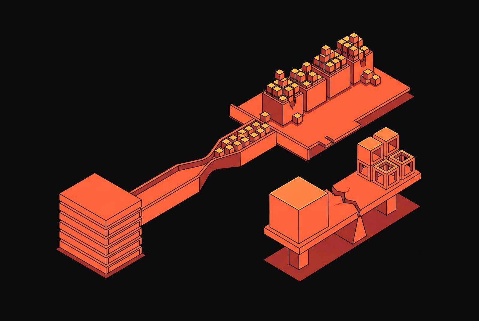
Open-source LLM inference stack benchmarking and optimization must account for GPU rental rates, KV cache growth, memory bandwidth, storage tiers, and network transport. Most open-source versus proprietary inference cost claims omit these variables and therefore cannot establish which option is cheaper at production scale. A valid comparison measures the full serving stack against the same context-length distribution, concurrency, and input/output mix.

Why most inference cost comparisons measure the wrong thing

The claim that “open-source is X times cheaper” usually compares GPU rental costs with proprietary per-token prices while leaving out the memory subsystem. These calculations name the GPU SKU, rental rate, and model weights, but treat VRAM capacity and storage bandwidth as fixed parts of the setup. They are not fixed in their effects. Context length, batch size, and KV cache behavior set how much useful work the rented hardware can do.

As a result, two deployments with the same models and GPU counts can have very different costs for the work they do. A per-token headline rate does not expose that difference when the underlying workload is unspecified. The omission invalidates the comparison for long-context or concurrent workloads because it removes the variables that determine serving capacity. Compute prices alone cannot establish an inference advantage.

What the KV cache actually is and why its memory footprint grows without bound

The key-value cache stores past token representations so that autoregressive generation can reuse them, saving the work of recomputation. Its memory requirement is expressed as KV_bytes = 2 × L × H_kv × D × S × B × bytes_per_element. Here, L is the layer count, H_kv is the number of key-value heads, D is the head dimension, S is the sequence length, and B is the batch size. The cache grows with the workload it serves. Layer count, head count, and head dimension come from the model architecture, while sequence length, batch size, and storage precision enter through serving conditions.

For a fixed architecture and precision, cache memory scales linearly with sequence length and batch size. Longer contexts thus use up memory that could hold more concurrent sequences. Model weights alone do not describe the footprint. The formula has no fixed cache allowance independent of workload, so any capacity estimate needs explicit limits on context and concurrency. This is why a model can fit in VRAM and still leave too little memory for the serving load it needs to handle.

Why decode throughput is bound by memory bandwidth, not FLOP count

Memory capacity determines what fits, while memory bandwidth determines how quickly decode can use it. Autoregressive decode has low arithmetic intensity because each step loads model weights and the full KV cache to produce a single token. In the roofline model, workloads below the hardware’s ridge point fall in the bandwidth-limited region. More arithmetic capacity does not remove that constraint. So a cost calculation based on peak FLOP throughput uses a level of performance that decode cannot reach.

This distinction is especially important for output-heavy workloads, where decode dominates token-generation latency and cost. Each output token needs another memory-bandwidth pass over weights and cache, while prefill uses resources differently as it processes the input. Providers reflect that asymmetry by charging significantly more for output tokens than input tokens. Blended token rates obscure the distinction. Two GPU configurations with the same FLOP count can consequently deliver different decode throughput because their HBM bandwidth or cache residency strategies differ.

How VRAM pressure collapses the throughput assumptions behind crossover-point calculations

The self-hosting crossover point is the token volume at which it costs less to run dedicated GPUs than to buy API access. Its calculation rests on an assumed throughput per GPU, often without specifying the context lengths that support that throughput. At very long context, an H100 with 80 GB VRAM can hold effectively one or two users’ KV cache alongside model weights. Concurrency is then constrained by cache capacity. A throughput estimate based on many more users at once is for a different workload from the one being priced.

As context grows, the crossover point therefore shifts with the loss of available serving capacity. Model size, infrastructure choices, and the input/output ratio already affect that point, but context length changes how much capacity those calculations can count on. Allocation behavior adds another source of error. Before PagedAttention, contiguous KV cache allocation wasted 60–80% of VRAM through fragmentation, leaving naive deployments with far less usable capacity than nominal memory suggested. Ignoring these effects does not merely understate infrastructure expense, but assigns the deployment a capacity profile it cannot sustain.

The three-tier storage hierarchy that cost comparisons don't include

When the cache needs more space than VRAM has, offloading moves it into a storage hierarchy whose bandwidth and latency set their own limits. A production 2026 inference node uses HBM for hot KV blocks, CPU DRAM for warm sessions and shared prefixes, and local NVMe for cold sessions and long-tail cache. Offloading preserves useful throughput or moves the bottleneck away from the GPU depending on the tiers' access costs.

HBM provides the highest bandwidth, at approximately 3.35 TB/s on H100 SXM5, but is the scarcest and most expensive tier per byte. CPU DRAM can supply multiple terabytes per 8-GPU node and acts as the cheapest available VRAM extension. The transfer path limits that apparent bargain. PCIe bandwidth between CPU and GPU constrains how quickly offloaded cache can return to the device, particularly under the workloads that put the most pressure on VRAM.

Local high-endurance NVMe provides 2–60+ TB for colder cache, with latency ranging from tens of microseconds to milliseconds. At 2026 context lengths, reloading cached state from NVMe can be faster and cheaper than recomputing prefill. Drive endurance, bandwidth, and PCIe lane allocation are procurement details that become part of the serving specification.

The strongest objection is that CPU DRAM offload is well understood and its direct cost is modest. That objection prices the memory but not the transfer penalty. Every decode step that touches offloaded cache is subject to the CPU-to-GPU bandwidth limit, which can reduce the output obtained from the same rented GPUs. The relevant cost is therefore not just dollars per GB, but the throughput lost while the memory subsystem supplies data.

What prefill-decode disaggregation adds to the infrastructure cost picture

Prefill-decode disaggregation makes the transport dependency explicit by placing the two phases in different serving groups. Prefill is compute-intensive and shapes time-to-first-token, while decode is memory-bandwidth-intensive and shapes time-per-output-token. Sharing a GPU does not optimally provision either phase. Separating them allows different resource allocations, but requires request-specific KV state to cross the backend network. What was a memory operation inside the GPU thus needs data transport, with infrastructure costs of its own.

Mooncake, Kimi’s production disaggregated system, implements an RDMA-based Transfer Engine with topology-aware path selection. Its transport reduced mean time-to-first-token compared with TCP, demonstrating that the network fabric affects serving performance independently of GPU count. SGLang’s 96-H100 deployment of DeepSeek-R1 used a 3-prefill, 9-decode node split. GPU allocation was only part of that configuration. Its throughput and cost profile also depended on the network fabric and NVMe tier, which a simple GPU-hours-to-API-price comparison would omit.

MLPerf Inference results treat disaggregation as a concrete benchmark configuration. Cisco’s submission paired NVIDIA H200 GPUs for prefill with AMD Instinct MI350X for decode, matching hardware to the distinct demands of the phases. MangoBoost achieved AMD GPUs’ first disaggregated inference submission in the MLPerf Inference v6.1 round. Software choices also changed the measured performance. NVIDIA improved its DeepSeek-R1 score substantially in the v6.0 cycle without changing hardware, using TensorRT-LLM kernel fusions and KV-aware routing through the Dynamo inference framework. These results make the serving configuration part of the evidence that must accompany the cost claim.

How KV cache optimizations shift the cost curve without appearing in cost comparisons

Even on the same hardware, cache optimization can decide whether long-context serving is worth its cost. PagedAttention in vLLM reduces fragmentation to under 4%, allowing more of the available VRAM to support useful cache. That changes the batch size a GPU can sustain and, with it, throughput. Allocation efficiency directly changes the cost curve. A comparison that names the model and GPU but omits the allocation strategy has not specified an equivalent deployment.

Attention architecture also makes a difference that serving software cannot remove. GQA-8, as used in Llama 3, reduces KV memory by a large fraction relative to standard MHA, while DeepSeek’s MLA reduces it further to a fraction of that baseline. Two models with the same parameter count can therefore have substantially different memory costs at long context. Parameter count alone cannot normalize the comparison.

Cache precision changes the footprint again. FP8 KV quantization cuts cache memory roughly in half, with accuracy loss within measurement noise for most production workloads. NVFP4 on Blackwell architecture reduces cache storage to 4-bit, making it meaningfully smaller than BF16. Because deployments differ in which of these options they have and use, a cost comparison must name the precision used in each, without assuming they share the same cache representation.

Weight compression can also release memory for cache. DFloat11 and ZipServ represent research directions in lossless coding of BF16 model weights, reducing the GPU memory footprint without accuracy loss. The freed memory can hold more KV cache, so the space used by weights affects serving concurrency. These techniques operate below the token-rate headline. Their presence or absence can change the economics even when the external API exposes the same input and output units.

How do you prove open-source inference is faster and cheaper at scale?

Context length must be reported as a distribution, including p50, p90, and p99 request lengths, because the tail drives memory pressure that an average conceals. Concurrent user count and session overlap must also be specified. The shape of the traffic changes how much shared prefixes help. Workloads with the same token volumes can have different prefix-cache hit rates and need different amounts of memory.

The serving configuration must then identify PagedAttention, prefix caching, GQA or MLA, quantization precision, and any lossless compression in use. Its infrastructure specification must include HBM capacity, CPU DRAM size, and NVMe endurance and bandwidth. Disaggregated deployments must also name the network fabric. These are inputs to the measured result. Without them, a claim about open-source versus proprietary inference is a compute price quote applied to a workload it was not measured against.

Performance results must also report time-to-first-token and time-per-output-token separately, while cost accounting must state the input/output ratio. Prefill and decode use different resources, so a blended rate is meaningful only for the workload mix behind it. FlexGen illustrates a more rigorous modeling approach. It estimates latency, bandwidth, and memory constraints for each device, including GPU, CPU, and disk, to determine placement of weights, activations, and KV cache. That approach puts a cost on the limits that shape execution, without assuming that all rented compute yields useful throughput.

Dell Technologies’ KV cache survey maps optimization techniques to seven practical deployment scenarios, including long-context single requests, high-throughput datacenter serving, multi-turn conversations, and accuracy-critical reasoning. No single technique or cost figure works across all of these settings. Benchmark conditions must follow the intended deployment. For production stacks running Llama, Qwen, or Mixtral, a benchmark cost survives real traffic only when KV cache residency, NVMe tier management, and high-throughput data movement support it. Open-source inference is demonstrably cheaper only when that full configuration delivers the claimed cost under the workload being compared.