GPU Utilization Benchmarking Methodology for LLM Inference
Separate prefill and decode measurements to expose compute versus memory constraints.

GPU utilization benchmarking for LLM inference fails when it treats the GPU as a single operating mode. A rigorous methodology must measure prefill and decode separately, because compute throughput constrains one while memory bandwidth constrains the other. Infrastructure decisions require phase-specific evidence about useful work, stalls, latency, and load.
Why a single GPU utilization number cannot characterize LLM inference
A practitioner runs nvidia-smi, reads the utilization figure, and uses it to judge how much more work a serving GPU can take on. That inference is flawed because the number does not identify the resource that limits the workload. A high reading during prefill and a lower reading during decode describe different execution regimes. Averaging them hides the distinction. The resulting figure is structurally misleading as a basis for capacity decisions.
The consequences extend beyond performance diagnosis. Chung et al. (2026) report 3–5× differences in energy use across GPU utilization levels, tied to how much memory is available, how much the hardware is used, and what the application needs. The utilization number exposes the symptom without explaining those factors. Patil (2026) finds that every public LLM cost calculator surveyed uses a fixed value for utilization without measuring it against the actual load. An ambiguous performance indicator therefore becomes an unsupported pricing assumption.
What prefill and decode actually do to a GPU
Prefill uses a large matrix multiply to process all prompt tokens in parallel. This gives the tensor cores enough arithmetic work to drive SM utilization high, making compute throughput the constraint. Decode instead generates one token per step. At small batch sizes, each step must read the full weight set and the KV cache built up so far from HBM to do relatively little arithmetic work. The GPU can consequently spend much of its time waiting for data.
Larger batches amortize weight reads across requests, so batch size matters to this distinction. TokenPowerBench (2025) attributes energy to the prefill and decode stages of every request through a phase-aligned pipeline, reflecting their distinct power signatures. WattGPU models inter-token latency separately from mean power draw and finds that GPU selection affects them differently. Hardware suitability therefore cannot be reduced to either power or activity alone.
How KV cache mechanics translate into a memory-bandwidth crisis during decode
The KV cache stores key and value vectors for every prior token. Each decode step reads the cache accumulated so far, making HBM read volume grow linearly with context length. The demand for memory thus changes through generation even with the same model and GPU. A sample taken early in generation therefore does not describe the conditions near its end. Decode is a moving target both within a single request and across different workloads.
At extended context lengths, a large model’s KV cache can exceed the capacity of a single GPU’s HBM. Spill to CPU DRAM or NVMe then changes the memory access pattern, so a shorter-context measurement no longer represents the same operating conditions. Chung et al. (2026) find order-of-magnitude differences in energy use across LLM task types, in part because of output length. That length also determines how far cache accumulation progresses during generation. Comparable decode measurements must therefore identify both the position in the sequence and the KV cache occupancy at that moment.
Why the standard profiling toolkit produces the wrong diagnosis
Standard SM-utilization reporting records activity. On its own, it cannot tell whether compute saturation or memory stalls account for the activity. A GPU can report high utilization while the work assigned to it spends most cycles waiting for HBM data. Conversely, low arithmetic throughput during decode need not mean that the hardware has unused capacity at its limiting resource. The dashboard presents a valid activity signal but leaves the bottleneck unresolved.
Model FLOPs Utilization, or MFU, measures the fraction of theoretical peak FLOP/s that the workload achieves. It can diverge sharply from SM utilization during decode because memory-bound activity produces little arithmetic relative to peak compute capacity. Yet end-to-end latency and a single utilization axis do not attribute losses to memory stalls, tile shape, CTA wave loss, occupancy caps, or instruction-set fragmentation. WattGPU finds substantial prediction error on unseen LLM-GPU combinations from load-scaled TDP power estimates and roofline latency estimates. Insufficiently discriminating instrumentation and models thus cause these diagnostic failures.
What a phase-aware, counter-pinned measurement methodology looks like
A defensible methodology starts with explicit phase boundaries in the serving framework. It records timestamps at prefill start, prefill end when the first token is generated, and decode completion. Hardware counter samples belong within those windows. Each counter must have verified semantics so that the reported metric means what its label claims. During decode, samples also need their corresponding KV cache occupancy to explain changing memory pressure.
MFU divides actual FLOP/s by theoretical peak and gives compute efficiency a consistent meaning across phases. Memory bandwidth utilization divides HBM read bytes per second by peak bandwidth and captures the primary decode constraint. Stall attribution reports the share of SM cycles spent in memory-dependency stalls, which NCU counter terminology calls long scoreboard stalls. Together, these measurements distinguish compute saturation from active execution that is waiting on memory.
Time to first token, or TTFT, should be reported at P50, P90, and P99 to expose prefill latency under realistic concurrency. Inter-token latency, or ITL, belongs in a separate decode report because each generation step depends on memory bandwidth and cache size. Energy measurements also need a clearly stated window of time. Chung et al. (2026) use vLLM 0.11.1 on NVIDIA H100 and B200 GPU nodes and calculate energy per token from the energy used and tokens generated during steady state. Identifying that interval prevents ramp-up behavior from silently determining the average.
How concurrency and offered load interact with phase-separated metrics
Request timestamps alone do not solve attribution under concurrent serving. Prefill from one request can overlap with decode from another on the same GPU, leaving device-level counters entangled even when each request has clear boundaries. The offered request rate, λ, determines how much of each phase is in flight. At low load, idle gaps can dominate, while at high load the phases overlap continuously. A benchmark must therefore describe the traffic conditions under which its phase metrics were collected.
Under Little’s Law, the mean number of requests in flight equals the arrival rate multiplied by the mean sojourn time. For comparisons that can be reproduced, λ must be stated and controlled at each measurement point, then swept across traffic levels that reflect production. Each point should report per-phase metrics and document the concurrency at which prefill and decode begin to interfere. Patil (2026) identifies offered load as the operator-controlled variable with the largest impact on effective utilization in a cost model that also includes hardware, model, quantization, and context length. WattGPU separately evaluates offline batch and online server scenarios and finds different prediction accuracy and GPU ranking correlations. Load regime is consequently part of the experiment.
What phase-separated measurement reveals about prefill-decode disaggregation
Prefill can saturate compute while decode is constrained by bandwidth, so a shared pool’s blended reading conceals inefficient use of the resource relevant to each phase. Dedicating compute-optimized capacity to prefill and bandwidth-optimized or power-capped capacity to decode is rational only when the measured profiles support it. Results for each phase must also guide how much capacity each pool gets.
Separation introduces a cost that the comparison cannot omit, namely the transfer of KV cache tensors between the pools. Transfer bandwidth depends on the interconnect, including NVLink within a domain, InfiniBand across nodes, and TCP across datacenters. That transfer latency must be included in the decode-phase TTFT budget. Chung et al. (2026) also find that increasing GPU count can sometimes reduce total energy by unlocking more memory capacity. Phase-level attribution makes that result interpretable by revealing where memory constrained execution. The decision rests on the measured balance of resource relief, transfer delay, and energy.
How quantization and precision format choices appear differently in each phase
Comparisons of higher-precision formats and FP8 also need measurements for each phase. During decode, reducing weight precision reduces the HBM bandwidth required per step and directly relieves the dominant bottleneck. During prefill, the benefit is smaller because weights serve a large matrix multiply whose constraint is compute throughput. A blended benchmark can therefore understate the decode latency benefit while overstating quantization as a general throughput lever. The reported gain depends on how much of the benchmark belongs to each phase.
FP8 KV cache makes the distinction especially clear. Halving the per-token KV memory footprint reduces the volume read on every decode step, so its benefit must be evaluated against decode-phase ITL. Chung et al. (2026) note that lower precision is not always faster or more energy efficient, reinforcing the need to identify the bottleneck before interpreting a format change. Patil (2026) finds that FP8 quantization benefits MoE architectures substantially more than dense models and identifies active parameter count, rather than total model size, as a primary predictor of saturation economics. Separate bandwidth and compute measurements make those differences visible instead of folding them into a single precision ranking.
Building a reproducible phase-aware benchmark protocol for production use
A production protocol turns these distinctions into a repeatable experimental record. Its design must combine phase boundary instrumentation, per-phase counter collection, production-representative load sweeps, decode cache occupancy tracking, and explicit steady-state identification. The record must specify the inference engine version, GPU model, precision format, and parallelism configuration exactly. These variables affect execution and cannot be relegated to optional metadata. Without them, a difference between runs cannot be attributed confidently to the change under examination.
The workload specification must give the input length distribution, output length distribution, and request arrival pattern. Fixed input and output lengths do not expose the variation in KV cache occupancy that governs real decode behavior. The load sweep must test more than one low-rate point so that it shows saturation and phase overlap. RunPod’s 2026 GPU benchmark explicitly states that it does not publish saturation runs and acknowledges the limits of its one-request-per-second methodology for measuring GPU behavior at higher concurrency. That distinction defines what a published comparison can support and what a production benchmark still needs to establish.
The final report must preserve the separation between prefill SM utilization and MFU, decode memory bandwidth utilization and ITL distribution, and stall attribution for both phases. It must separate steady state from ramp-up before working out the averages for energy or utilization. TokenPowerBench (2025) demonstrates that phase-aligned measurement across GPU, node, and rack granularity is achievable in open-source tooling without specialized power meters. Storage and memory instrumentation must complete that record by documenting KV cache I/O through HBM, CPU DRAM, or NVMe. Those layers feed data to decode, so a benchmark that assumes they stay fixed would leave the main bottleneck unmeasured.
Sources
- TokenPowerBench: Benchmarking the Power Consumption of LLM Inference
- WattGPU: Predicting Inference Power and Latency on Unseen GPUs and LLMs
- Where Do the Joules Go? Diagnosing Inference Energy Consumption
- Beyond Per-Token Pricing: A Concurrency-Aware Methodology for LLM Infrastructure Cost Estimation
- Characterization of Request and Token Energy Costs for LLM Inference Workloads on GPU Platforms
- Dissecting GPU Utilization for LLM Inference on Nvidia Hopper